This content is from the fall 2016 version of this course. Please go here for the most recent version.
Homework 05: Analyzing the gapminder dataset using Python
Overview
Due before class Wednesday November 2nd.
The basic goal of the assignment is to implement various computational methods (e.g. data frames, lists, filtering, conditional expressions, iteration, functions) in Python. Rather than using raw programming assignments, you will demonstrate these skills in the context of analyzing the gapminder dataset, something you have already explored in R.
Fork the hw05 repository
Go here to fork the repo for homework 05.
Workflow
You are provided with a Jupyter Notebook similar to the one seen here. Fill in the chunks with the appropriate code needed to perform the requested analysis. I have already identified the questions and tasks you need to perform.
Submit the assignment
Your assignment should be submitted as a single Jupyter Notebook. Follow instructions on homework workflow. As part of the pull request, you’re encouraged to reflect on what was hard/easy, problems you solved, helpful tutorials you read, etc.
Rubric
Check minus: Notebook cannot be run. Didn’t answer all of the questions. Code is incomprehensible or difficult to follow.
Check: Solid effort. Hits all the elements. No clear mistakes. Easy to follow (both the code and the output). Nothing spectacular, either bad or good.
Check plus: Innovative use of coding elements to solve the problems (e.g. functions, conditional expressions, iterations). Adds labels to graphs. Uses techniques beyond those from the example notebooks. Successfully attempts the advanced challenge.
Import packages and setup the notebook
# Import libraries
import pandas as pd
import numpy as np

# Turn off notebook package warnings
import warnings
warnings.filterwarnings('ignore')

# print graphs in the document
%matplotlib inline
Load the data with Pandas
Print the first five rows of the gapminder DataFrame
What is the average (mean) life expectancy for the entire dataset?
59.474439366197174What is the average (mean) life expectancy, for each continent?
continent
Africa      48.865330
Americas    64.658737
Asia        60.064903
Europe      71.903686
Oceania     74.326208
Name: lifeExp, dtype: float64
For each country in Oceania, print the subset of the data for that country
Australia
      country continent  year  lifeExp       pop    gdpPercap
60  Australia   Oceania  1952   69.120   8691212  10039.59564
61  Australia   Oceania  1957   70.330   9712569  10949.64959
62  Australia   Oceania  1962   70.930  10794968  12217.22686
63  Australia   Oceania  1967   71.100  11872264  14526.12465
64  Australia   Oceania  1972   71.930  13177000  16788.62948
65  Australia   Oceania  1977   73.490  14074100  18334.19751
66  Australia   Oceania  1982   74.740  15184200  19477.00928
67  Australia   Oceania  1987   76.320  16257249  21888.88903
68  Australia   Oceania  1992   77.560  17481977  23424.76683
69  Australia   Oceania  1997   78.830  18565243  26997.93657
70  Australia   Oceania  2002   80.370  19546792  30687.75473
71  Australia   Oceania  2007   81.235  20434176  34435.36744
New Zealand
          country continent  year  lifeExp      pop    gdpPercap
1092  New Zealand   Oceania  1952   69.390  1994794  10556.57566
1093  New Zealand   Oceania  1957   70.260  2229407  12247.39532
1094  New Zealand   Oceania  1962   71.240  2488550  13175.67800
1095  New Zealand   Oceania  1967   71.520  2728150  14463.91893
1096  New Zealand   Oceania  1972   71.890  2929100  16046.03728
1097  New Zealand   Oceania  1977   72.220  3164900  16233.71770
1098  New Zealand   Oceania  1982   73.840  3210650  17632.41040
1099  New Zealand   Oceania  1987   74.320  3317166  19007.19129
1100  New Zealand   Oceania  1992   76.330  3437674  18363.32494
1101  New Zealand   Oceania  1997   77.550  3676187  21050.41377
1102  New Zealand   Oceania  2002   79.110  3908037  23189.80135
1103  New Zealand   Oceania  2007   80.204  4115771  25185.00911
Sort gapminder by population. Make sure the sorted object replaces the existing gapminder DataFrame
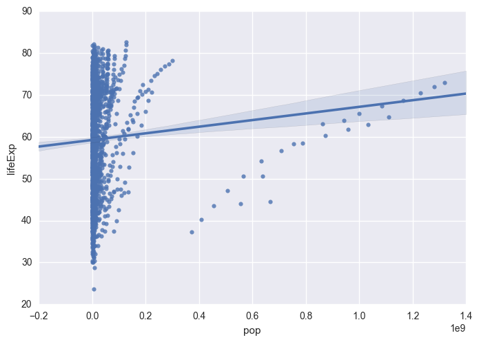
Using seaborn, generate a scatterplot depicting the relationship between population and life expectancy and include a linear best fit line
import seaborn as sns<matplotlib.axes._subplots.AxesSubplot at 0x10833b2b0>
png
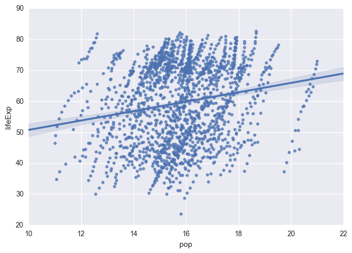
Generate the same graph as above, but this time log-transform the population variable
<matplotlib.axes._subplots.AxesSubplot at 0x108450518>
png
Write a Function
(To Assess the Relationship Between Year and Life Expectancy for a Given Country)
Here the goal is to write a basic function, “life_expectancy”, that incorporates your work above.
By default, the function should return a scatterplot of life-expectancy versus years for a given country. [Hint: Subset the data for a specific country, similar to a problem above]
Once you subset the data, the function should do one of two things: * (1) return a graph [or] * (2) return a graph and model results.
Thus, your function should have arguments and output as follows:
*   Arguments:
        Country (required):   The name of a specific country, such as "Australia"
        Model   (optional):   Build and Return a Model Results, #Hint, set the default to be False

*   Output:
        (1) - Default: A scatterplot of the relationship with best fit line
        (2) - Model:   The above graph AND the model results
Of course, we have not yet covered modeling in Python.
To run a linear model, we can use the library statsmodels, to predict life expectancy by year.
Example for this problem:
import statsmodels.formula.api as sm #Import Package
model = sm.ols(formula = 'lifeExp ~ year', data = gapminder).fit() #Fit OLS Model
results = model.summary() #Get Results
print(results) # Print

#Hint: Use this Code in Your Function.
#You will need to replace data = gapminder, with the data subset for a specific country.
OLS Regression Results
==============================================================================
Dep. Variable: lifeExp R-squared: 0.190
Model: OLS Adj. R-squared: 0.189
Method: Least Squares F-statistic: 398.6
Date: Tue, 25 Oct 2016 Prob (F-statistic): 7.55e-80
Time: 16:40:53 Log-Likelihood: -6597.9
No. Observations: 1704 AIC: 1.320e+04
Df Residuals: 1702 BIC: 1.321e+04
Df Model: 1
Covariance Type: nonrobust
==============================================================================
coef std err t P>|t| [95.0% Conf. Int.]
------------------------------------------------------------------------------
Intercept -585.6522 32.314 -18.124 0.000 -649.031 -522.273
year 0.3259 0.016 19.965 0.000 0.294 0.358
==============================================================================
Omnibus: 386.124 Durbin-Watson: 1.962
Prob(Omnibus): 0.000 Jarque-Bera (JB): 90.750
Skew: -0.268 Prob(JB): 1.97e-20
Kurtosis: 2.004 Cond. No. 2.27e+05
==============================================================================
Warnings:
[1] Standard Errors assume that the covariance matrix of the errors is correctly specified.
[2] The condition number is large, 2.27e+05. This might indicate that there are
strong multicollinearity or other numerical problems.# write your function hereExample Results for the Function
Your function should be able to produce these results:
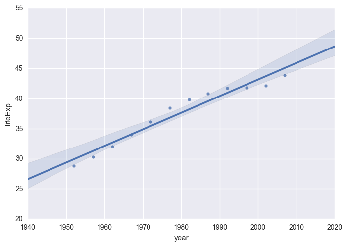
# Result for a Country (No Model)
life_expectancy("Afghanistan")
png
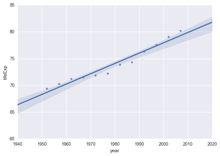
# Result for a Country (Model = True)
life_expectancy("New Zealand", True)
OLS Regression Results
==============================================================================
Dep. Variable: lifeExp R-squared: 0.954
Model: OLS Adj. R-squared: 0.949
Method: Least Squares F-statistic: 205.4
Date: Tue, 25 Oct 2016 Prob (F-statistic): 5.41e-08
Time: 16:49:02 Log-Likelihood: -13.321
No. Observations: 12 AIC: 30.64
Df Residuals: 10 BIC: 31.61
Df Model: 1
Covariance Type: nonrobust
==============================================================================
coef std err t P>|t| [95.0% Conf. Int.]
------------------------------------------------------------------------------
Intercept -307.6996 26.630 -11.554 0.000 -367.036 -248.363
year 0.1928 0.013 14.333 0.000 0.163 0.223
==============================================================================
Omnibus: 1.899 Durbin-Watson: 0.530
Prob(Omnibus): 0.387 Jarque-Bera (JB): 1.086
Skew: -0.420 Prob(JB): 0.581
Kurtosis: 1.789 Cond. No. 2.27e+05
==============================================================================
Warnings:
[1] Standard Errors assume that the covariance matrix of the errors is correctly specified.
[2] The condition number is large, 2.27e+05. This might indicate that there are
strong multicollinearity or other numerical problems.
png
Advanced Challenge (Optional)
Assess the relationship between year and life expectancy
As you know already, the general trend is that over time life expectancy increases, but the trend is different for each country. Some experience a greater increase than others, whereas some countries experience declines in life expectancy. You can use whatever method you wish to assess and explain this relationship using Python.
- You could draw a graph
- You could draw a graph which visualizes the differing relationships between countries
- You could estimate a correlation coefficient
- You could estimate a statistical model - note that the notebook as written uses Python 2. For the most part it works with Python 3 though.
- You could estimate a statistical model for each country
Use whichever method you think you can master before the assignment is due. Some of you may just stick to basic graphs and tables, while others might build a statistical model using statsmodel. Obviously the more advanced technique you use, the higher your ceiling will be for your evaluation. But don’t spend 10 hours getting this to work! Go with what you can accomplish in a reasonable amount of time.
This work is licensed under the CC BY-NC 4.0 Creative Commons License.