Python

Python was developed in the 1990s as a general-purpose programming language. It emphasizes simplicity over complexity in both its syntax and core functions. As a result, code written in Python is (relatively) easy to read and follow as compared to more complex languages like Perl or Java. This also means the base installation of Python is actually very minimalistic - to perform data analysis of any significance, you will almost assuredly have to use an add-on library.

Python 2 or 3?

tl;dr - use Python 3

When software is updated, developers typically try to avoid breaking pre-existing features. So a version update from 2.2 to 2.3 typically includes minor changes which allow previously written code to (mostly) continue working correctly. Sometimes however updates are so significant and expansive that they break existing code. When this happens, developers typically signify such a transition by incrementing the base version number (i.e. instead of 2.2 -> 2.3, 2.2 -> 3.0).

Such a transition occured for Python in 2008 when Python 2.x was replaced by Python 3.0. Support for 2.x continued until 2010 with the final release in the 2.x line (2.7). Python 3.5 is the most recent major release and is considered the active development version. However because the switch from 2 -> 3 broke many existing libraries and functions, it has taken a large amount of time for major developers and libraries to make the transition to 3.x.

In this course we will use Python 3. It is the future of Python and for our purposes does what we need it to do. At some point in the future you may encounter a problem where you need to use a library that only works on Python 2. Or, more likely, you will find a Python script online that you want to repurpose only to find out it was written in Python 2 and you are now forced to rewrite for Python 3. When you reach this point, I wish you good luck and godspeed. Just kidding, the differences between Python 2 and 3 are not insurmountable, we just won’t cover them in this course. You can learn more about that on your own.

Anaconda

One approach to setting your machine up to program in Python would be the following:

1. Download Python and install.
2. Download an integrated development environment (IDE) in which to write and execute code (or just use a text editor).
3. Begin writing programs only to discover that you need to download and install a separate library using pip, PyPI or some other package manager to perform your analysis. Or worse, have to compile each library manually.
4. Go do this 50 separate times.
5. Become aggravated when libraries don’t install correctly.
6. Throw your computer out the window.

An alternative is to use Anaconda, an open-source distribution of Python which includes many useful packages pre-installed, a package manager to download and install over 700 additional packages, and some additional applications built on Python, one of which we will find very useful.

Jupyter Notebook

Juypter (formerly iPython) Notebook is a popular IDE for writing and executing Python scripts. Jupyter Notebook is actually a web server (run either locally or on the internet) that runs Python, R, and other popular computer languages and combines live code with output and explanatory text to integrate your workflow. The result is a single reproducible document which contains your research and analysis. Jupyter Notebook is installed with Anaconda.

Test it

Make sure you’ve installed everything correctly.

1. Run jupyter notebook from the shell (using Terminal in Mac/Linux or the Command Prompt in Windows). You should see some output like this:

$ jupyter notebook
[I 08:58:24.417 NotebookApp] Serving notebooks from local directory: /Users/benjamin
[I 08:58:24.417 NotebookApp] 0 active kernels
[I 08:58:24.417 NotebookApp] The Jupyter Notebook is running at: http://localhost:8888/
[I 08:58:24.417 NotebookApp] Use Control-C to stop this server and shut down all kernels (twice to skip confirmation).

Most of this information is not directly relevant for our purposes, but one important thing it tells us is the URL of your local notebook server (by default, http://localhost:8888). Running jupyter notebook also automatically launches the server in your default web browser.

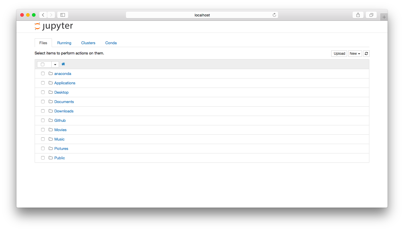
The Notebook Dashboard should open in your web browser. From here you can navigate directories and files, and create and open notebooks.

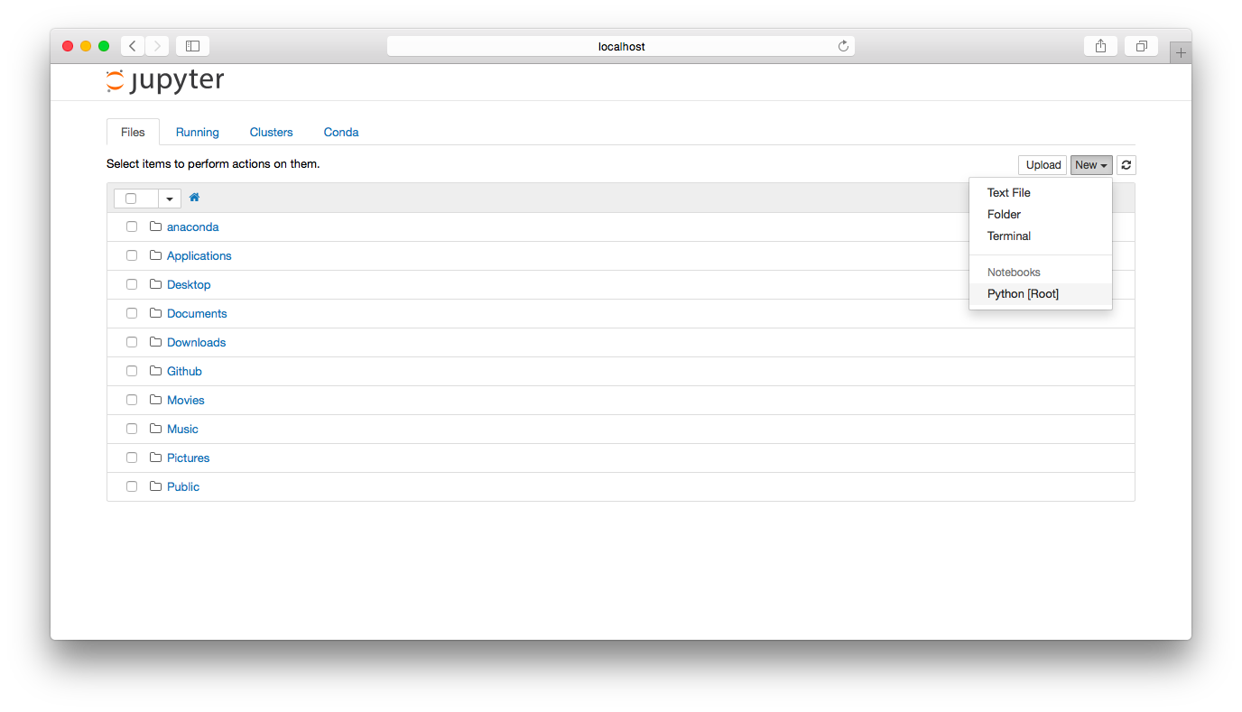
To make sure you’ve set everything up correctly, click “New” > “Notebooks (Python)”.

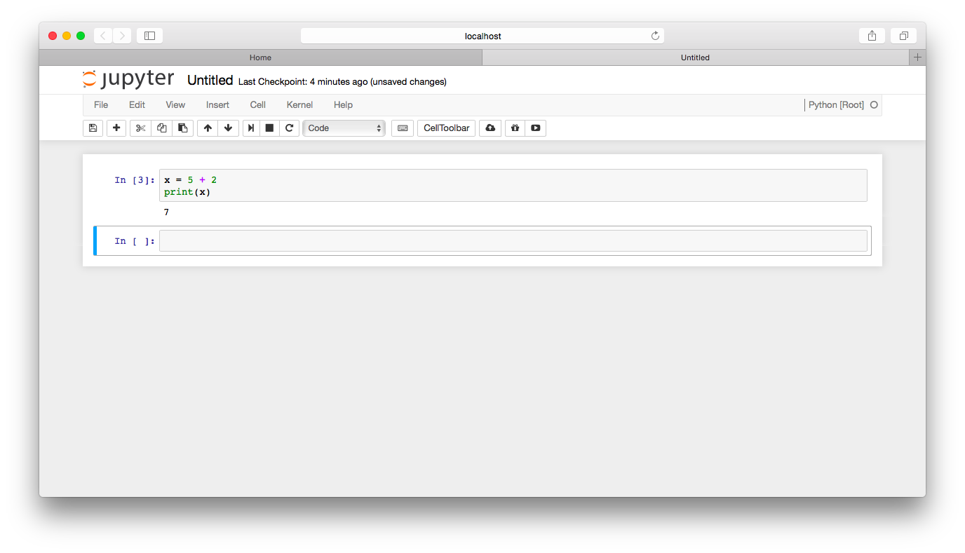
You’ve just created a new notebook in the directory where you launched jupyter notebook. In the future, you can store notebooks in any directory you prefer using the Notebook Dashboard. Now, type the following code in the first cell and then press Shift + Enter.

x = 5 + 2
print(x)

Your window should now look like this:

If done correctly, you’ve just performed basic arithmetic, stored the result in an object, then printed the object to your screen.

To close your notebook, close the browser windows for your Jupyter Notebook and the Notebook Dashboard. Then back in the command line window, type Control-C twice to stop the Notebook server.